February 21, 2016
As with most topics in Machine Learning, State Space Modeling is a general concept used to construct more complex models.The concept of State Space modeling is the following: We are given a set of observations (samples) \(x_t\). In lieu of defining a statistical model directly on the observations - we view them as noisy (errorful, partial) observations of some underlying state \(\mu_t\) by defining a probability model that relates observations to states. We then specify a model on the states \(\mu_t\).
As this is a natural concept it shows up in various fields in different guises, using different terminology, and different algorithms. In this post we will explore state space modelling using examples and along the way make connections between it’s varied uses.
The ingredients for a state space model are roughly the following.
A sample space \(\mathcal{X}\) to represent our measurements
A sample space \(\mathcal{Y}\) to represent our states.
A probability distribution on \(\mathcal{X} \times \mathcal{Y}\) that represents the probability our making observation \(x\) given that the true state is \(y\).
A model for the states.
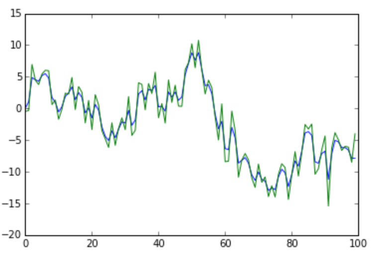
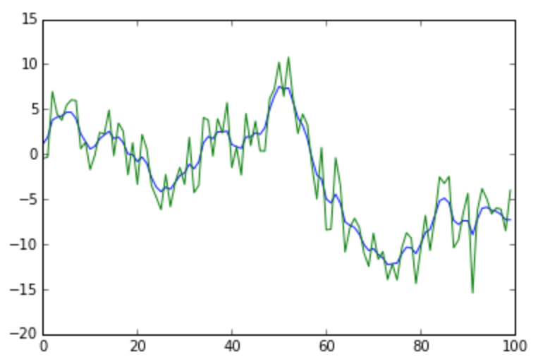
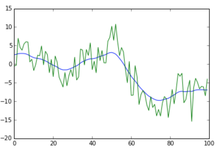
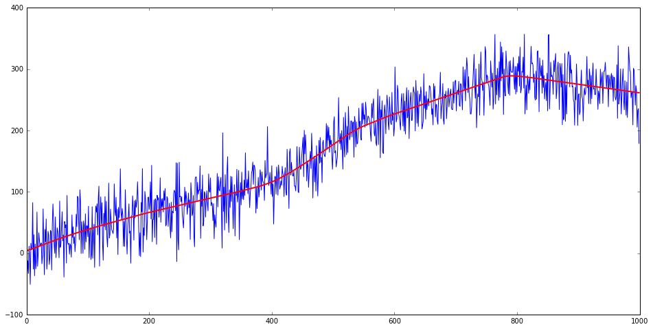
We start with the most elementary example of a continuous state space model. We have a set of \(T\) measurements taken over time, \(x_t \in \mathbb{R}\), which we assume derive from states \(\mu_t\) which are nearly constant.
Ingredients:
Measurement sample space : \(\mathbb{R}\)
State sample space: \(\mathbb{R}\)
Measurement Model : Errors \(x_t - \mu_t\) are independently normally distributed with mean 0 and standard deviation \(\sigma_\epsilon\).
\[\begin{aligned} x_{t} &= \mu_t + \epsilon_t . \\ \epsilon_t &\sim N(0,\sigma_\epsilon^2)\quad \mathrm{i.i.d.}\end{aligned}\]
State Model : Time differences of states are independent normal distributed with mean 0 and standard deviation \(\sigma_\nu\)
\[\begin{aligned} \mu_t &= \mu_{t-1} + \nu_t \\ \nu_t &\sim N(0,\sigma_\nu^2) \quad \mathrm{i.i.d}\end{aligned}\]
All together this defines a probability distribution on the sample space of pairs of time-series (T long vectors) \(x_t\) and \(\mu_t\).
\[\begin{equation} \rho[\sigma_\nu,\sigma_\epsilon](x, \mu) = \prod_{t=1}^T \frac{1}{\sqrt{2\pi}\sigma_\epsilon} e^{-(x_t - \mu_t)^2/2\sigma_\epsilon^2} \prod_{t=1}^{T-1} \frac{1}{\sqrt{2\pi}\sigma_\nu} e^{-(\mu_{t+1} - \mu_t)^2/2\sigma_\nu^2} \end{equation}\]
Given observation for \(x_t\) we want to get a best estimate of the underlying states \(\mu_t\). First given an observation for \(x_t\) we can restrict our probability distribution to these observed values, or \(P(\mu \| x)\).
This involves fixing the values \(x\) in the above density to be the our observed values and determining a new normalization constant \(Z\) by integrating over \(\mu\).
\[\begin{equation} \rho[\sigma_\nu, \sigma_\epsilon](\mu \vert x) = \frac{1}{Z(\sigma_\epsilon, \sigma_\nu, x)}\, \rho[\sigma_\nu^2, \sigma_\epsilon^2](x, \mu) \end{equation}\]
A natural direction to take is looking for the maxima of this density - or simpler extreme values of the log of the density.
\[\begin{equation} \sum_{t=1}^T (x_t - \mu_t)^2/2\sigma_\epsilon^2 + \sum_{t=1}^{T-1} (\mu_{t+1} - \mu_t)^2/2\sigma_\nu^2 + \log{Z} \end{equation}\]
\(\mu_t\) are our free variables here - so we look for the \(\mu_t\) that minimizes this expression. Varying the density with respect to \(\mu_t\) we get the following set of equations.
\[\begin{aligned} (x_1 - \mu_1)/\sigma_\epsilon^2 + (\mu_{2} - \mu_1)/\sigma_\nu^2 &= 0 \quad \text{for}\quad t=1 \\ (x_t - \mu_t)/\sigma_\epsilon^2 + (\mu_{t+1} - 2\mu_t + \mu_{t-1} )/\sigma_\nu^2 &= 0 \\ (x_T - \mu_T)/\sigma_\epsilon^2 - (\mu_{T} - \mu_{T-1})/\sigma_\nu^2&= 0 \quad \text{for}\quad t=T\end{aligned}\]
Which is the following tri-diagonal system. Where we have defined
\(\lambda = \sigma_\epsilon^2/\sigma_\nu^2\).
\[\begin{equation} \begin{bmatrix} 1+ \lambda & -\lambda & 0 & \dots & 0 & 0 \\ -\lambda & 1+ 2\lambda & -\lambda & \dots & 0 & 0 \\ \vdots & \vdots & \vdots & \vdots & \vdots & \vdots \\ 0 & 0 & 0 & \dots & -\lambda & 1+ \lambda \end{bmatrix} \cdot \begin{bmatrix} \mu_1 \\ \mu_2 \\ \vdots \\ \mu_T \end{bmatrix} = \begin{bmatrix} x_1 \\ x_2 \\ \vdots \\ x_T \end{bmatrix} \end{equation}\]
There is a simple algorithm for tridiagonal linear systems. We first define \(a_i\) and \(b_i\) recursively (comes from an LU decomp).
\[\begin{aligned} \alpha_1 &= \frac{-1}{1+ \sigma_\nu^2/\sigma_\epsilon^2} = \frac{-\lambda}{1+\lambda} \\ \alpha_i &= \frac{-1}{\sigma_\nu^2/\sigma_\epsilon^2+ 2 + \alpha_{i-1}} = \frac{-\lambda}{1+2\lambda+\lambda\alpha_{i-1}} \\ \beta_1 &= \frac{x_1}{1 + \sigma_\epsilon^2/\sigma_\nu^2} = \frac{x_1}{1 + \lambda} \\ \beta_i &= \frac{x_i + \lambda \beta_{i-1}}{1 + 2\lambda + \lambda\alpha_{i-1}} \end{aligned}\]
Given these - \(\mu_i\) are obtained as follows.
\[\begin{aligned} \mu_n &= \beta_n \\ \mu_i &= \beta_i - \alpha_i \mu_{i+1}\end{aligned}\]
The initial representation as a state space model was far more transparent in terms of what we expect the output states to look like. At this stage the solution is quite opaque!
Example outputs for different values of \(\lambda\). As \(\lambda = \sigma_\epsilon^2/\sigma_\nu^2\) increases, the state noise \(\sigma_\nu\) shrinks relative to the measurement noise \(\sigma_\epsilon\) — the model trusts the state dynamics more and the estimated states become smoother. At large \(\lambda\) the estimated state is nearly a straight line; at small \(\lambda\) it tracks the observations closely.


There is an alternative derivation that gives a cleaner interpretation of \(\lambda\) — and reveals the local level smoother as simply a Fourier filter in disguise. Looking at the linear system of equations above - they are extremely close to being the following.
\[\begin{equation}(1+\lambda (2 - S - S^{-1}))\mu = \Lambda' \mu = x\end{equation}\]
Where \(S\) is a circular shift operator. \(Sx_t=x_{t+1}\). With the exceptions being the equations for the end-points. I have no idea if the following can be generalized, but notice that if we embed \(\mathbb{R}^T\) in \(\mathbb{R}^{2T}\) via a map \(\phi\) defined as.
\[\begin{aligned} \phi(x)_i = x_{i} \quad i = 1 \cdots T \\ \phi(x)_i = x_{2T+1-i} \quad i = T+1 \cdots 2T\end{aligned}\]
Or in other words we append the mirror reverse to the original. Then
The space of such mirror symmetric vectors is preserved by the operator above (so the inverse preserves it as well)
Restricting the \(\Lambda\) to these symmetric vectors and then looking at the first half of the vector - we have our original of equations.
It is the case that \(\phi^{-1} \Lambda \phi\) is our original matrix.
So we map \(x\) into \(R^{2T}\) via \(\phi\) invert the simple operator - and then apply the inverse \(\phi^{-1}\) (just take the first half of the vector) to get the solution. What makes this nice is that the operator can be simply inverted via Fourier transform.
\[\begin{equation} \frac{1}{1 + \lambda(2 - e^{2\pi i p/2T} - e^{-2\pi i p/2T})} \widetilde{\phi(x)}_p \end{equation}\]
In this expression we see the local level smoother as being simply a Fourier smoother - and \(\lambda\) picks up a simple interpretation as determining at which time-scale (or frequency) the damping of Fourier modes kicks in.
(This is hard to generalize beyond simple systems - there is a complex dance between the requirements that the new operator preserves the embedding and that the new operator restricts to the original)
Part I found the most probable full history of states given all \(T\) observations at once — a batch problem. The Kalman filter solves a different problem: the marginal distribution of the current state given only the observations so far, updated recursively as new observations arrive.
Concretely: Part I gives \(\arg\max_\mu P(\mu_1,\ldots,\mu_T \mid x_1,\ldots,x_T)\). The Kalman filter maintains \(P(\mu_t \mid x_1, \ldots, x_t)\) as a running estimate, never revisiting past observations.
Still starting from.
\[\begin{equation} \rho[\sigma_\nu, \sigma_\epsilon](x, \mu) = \prod_{t=1}^T \frac{1}{\sqrt{2\pi}\sigma_\epsilon} e^{-(x_t - \mu_t)^2/2\sigma_\epsilon^2} \prod_{t=1}^{T-1} \frac{1}{\sqrt{2\pi}\sigma_\nu} e^{-(\mu_{t+1} - \mu_t)^2/2\sigma_\nu^2} \end{equation}\]
If we have a set of observations \(x_1, x_2, ... x_t\) with t <=T. We can look at the probability of having a history of states given these observations. Requires two steps : conditioning on the observations \(x_1, x_2, .., x_t\) and marginalize / integrate out the rest of \(x_t\). Or another way to think of this - is to say that our sample space at time \(t\) is Only series up to \(t\) - so the sample space and distribution evolve with time.
\[\begin{equation} P(\mu_1, \mu_2, ..., \mu_t | x_1, x_2, ..., x_t) \end{equation}\]
The Kalman filter is computing.
\[\begin{equation} P(\mu_t | x_1, x_2, ..., x_{t-1}) = N(a_t, P_t)(\mu_t) \end{equation}\]
A nice side effect of having all Normal distributions is that the space of Gaussian functions is closed under tons of operations - so this probability distribution is normal at each step.
The Gaussian integrals involved use the identities collected at the end of this section. One can check that
\[\begin{aligned} P(\mu_t | x_1, \ldots, x_{t-1}) &= \int d\mu_{t-1}\, P(\mu_{t-1} | x_1, \ldots, x_{t-2}) \\ &\quad\cdot \frac{1}{\sqrt{2\pi}\sigma_\epsilon} e^{-(x_{t-1} - \mu_{t-1})^2/2\sigma_\epsilon^2} \cdot \frac{1}{\sqrt{2\pi}\sigma_\nu} e^{-(\mu_{t} - \mu_{t-1})^2/2\sigma_\nu^2} \\[6pt] &= \int d\mu_{t-1}\, \frac{1}{\sqrt{2\pi P_{t-1}}} e^{-(a_{t-1} - \mu_{t-1})^2/(2P_{t-1})} \\ &\quad\cdot \frac{1}{\sqrt{2\pi}\sigma_\epsilon} e^{-(x_{t-1} - \mu_{t-1})^2/2\sigma_\epsilon^2} \cdot \frac{1}{\sqrt{2\pi}\sigma_\nu} e^{-(\mu_{t} - \mu_{t-1})^2/2\sigma_\nu^2} \end{aligned}\]
Which gives the following update
\[\begin{aligned} a_{t} &= \frac{P_{t-1} x_{t-1} + a_{t-1} \sigma_{\epsilon}^2}{P_{t-1} + \sigma_{\epsilon}^2} = \frac{a_{t-1}/P_{t-1} + x_{t-1}/\sigma_{\epsilon}^2}{1/P_{t-1} + 1/\sigma_{\epsilon}^2}\\ P_t &= \sigma_\nu^2 + \frac{P_{t-1} \sigma_{\epsilon}^2}{P_{t-1} + \sigma_{\epsilon}^2} = \sigma_\nu^2 + \frac{1}{1/P_{t-1} + 1/\sigma_{\epsilon}^2} \end{aligned}\]
\[\begin{aligned} &\int dx\, \frac{1}{\sqrt{2\pi}\sigma} \frac{1}{\sqrt{2\pi}\rho}\, e^{-\frac{1}{2}(x-\mu)^2/\sigma^2}\, e^{-\frac{1}{2}(x-\nu)^2/\rho^2} \\ &= \frac{1}{\sqrt{2\pi(\sigma^2 + \rho^2)}}\, e^{-\frac{1}{2}(\mu-\nu)^2/(\sigma^2+\rho^2)} \end{aligned}\]
Denoting as \(N(\mu, \sigma^2)(x)\)
\[\begin{aligned} &\int dx\, N(\mu, a^2)(x)\, N(\nu, b^2)(x)\, N(\lambda, c^2)(x) \\ &= \frac{1}{2\pi abc\sqrt{1/a^2+1/b^2+1/c^2}} \\ &\quad\cdot \exp\!\left( -\frac{(\mu-\lambda)^2/a^2c^2 + (\mu-\nu)^2/a^2b^2 + (\nu-\lambda)^2/b^2c^2} {2(1/a^2+1/b^2+1/c^2)} \right) \end{aligned}\]
A common problem (for me) is the following extension. As opposed to having a uniform \(\sigma\) across all time - we often have error estimates per time \(\sigma_t\).
The probability model is nearly identical
Measurement Model : Errors \(x_t -\mu_t\) are independently normally distributed with mean 0 and standard deviation \(\sigma_\epsilon\). \[\begin{aligned} x_{t} = \mu_t + \epsilon_t . \\ \epsilon_t \sim N(0,\sigma_t^2)\quad \mathrm{i.i.d.}\end{aligned}\]
State Model : Time differences of states are independent normal distributed with mean 0 and standard deviation \(\sigma_\nu\) \[\begin{aligned} \mu_t = \mu_{t-1} + \nu_t \\ \nu_t \sim N(0,\sigma_\nu^2) \quad \mathrm{i.i.d}\end{aligned}\]
There are minimal changes to the method of solution.
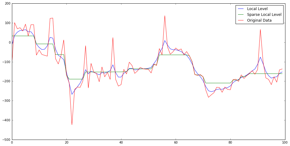
Looking at the local level smoother as an optimization problem we have a quadratic penalty on the first derivative of the state and a quadratic penalty on deviations of the observation from state. The max probability state history is a smooth curve that has small but non-zero derivative.
It does not quite live up to it’s "Local Level" name though, since the output time series are anything but locally constant. If we desire a first derivative that is mostly zero (sparse) intuition leads us to change the quadratic penalty on derivatives to an \(L_1\) as in Lasso.
It is simplest to jump directly to the optimization problem where we specify the following cost function (for state \(\mu\) given measurements \(x\))
\[\begin{equation} C(\mu, x) = \lambda \sum_{t=2}^T |\mu_{t} - \mu_{t-1}| + \sum_{t=1}^T (\mu_t - x_t)^2 \end{equation}\]
This can be molded into a Lasso linear regression problem but considering the values \(v_t = \mu_{t} - \mu_{t-1}\) to be coefficients and rewrite the quadratic term in terms of these variables.
\[\begin{equation} C(\mu, x) = \lambda \sum_{t=2}^T |v_t| + \sum_{t=1}^T \left(\mu_1 + \sum_{t'=2}^t v_{t'}- x_t\right)^2 \end{equation}\]
Where we now have a linear model with intercept \(\mu_1\) with input/output pairs : \(([0,0,\cdots,0,0],x_1), ([1,0,\cdots,0,0],x_2), ([1,1,\cdots,0,0],x_3)\), \(\cdots , ([1,1,\cdots,1,0],x_{T-1}), ([1,1,\cdots,1,1],x_T)\). Where the input vectors are length \(T-1\).

In going to an \(L_1\) penalty on the first derivative - we have broken the scale invariance of the cost function, so the size of the input data becomes important.
Probability interpretation? From the cost function we have the following
\[\begin{equation} x_t - \mu_t \sim N(0,\sigma^2) \end{equation}\]
\[\begin{equation} |\mu_t - \mu_{t-1}| \sim \mathrm{Exponential}(\lambda) \end{equation}\]
So overall probability
\[\begin{equation} \rho[\sigma_\nu, \sigma_\epsilon](x, \mu) = \prod_{t=1}^T \frac{1}{\sqrt{2\pi}\sigma} e^{-(x_t - \mu_t)^2/2\sigma^2} \prod_{t=2}^{T} \lambda\, e^{-\lambda |\mu_{t} - \mu_{t-1}|} \end{equation}\]
Resulting in likelihood (which shifts by a constant depending on measurements when we condition on \(x\)).
\[\begin{equation} C(\mu, x) = \lambda \sum_{t=2}^T |\mu_{t} - \mu_{t-1}| + \frac{1}{2\sigma^2} \sum_{t=1}^T (\mu_t - x_t)^2 - (T-1) \ln(\lambda) + T\ln(\sigma) \end{equation}\]
Again simplest to jump directly to the optimization problem where we specify the following cost function (for state \(\mu\) given measurements \(x\))
\[\begin{equation} C(\mu, x) = \lambda \sum_{t=3}^T |\mu_{t} - 2\mu_{t-1}+\mu_{t-2}| + \sum_{t=1}^T (\mu_t - x_t)^2 \end{equation}\]
This can be molded into a Lasso linear regression problem but considering the values \(a_t = \mu_{t} - 2\mu_{t-1}+\mu_{t-2}\) and \(v_2 = \mu_2 - \mu_1\) to be coefficients, \(x_1\) intercept and rewrite quadratic term in terms of these variables.
\[\begin{equation} C(\mu, x) = \lambda \sum_{t=3}^T |a_t| + \sum_{t=1}^T (\mu_t(\mu_1, v_2, a) - x_t)^2 \end{equation}\]
Where we read of the ‘inputs’ from linear relations between \(\mu_t\) and \(x_1,v_2,a_t\) as above.
\[\begin{aligned} \mu_2 &= \mu_1 + v_2 \\ \mu_3 &= \mu_1 + 2v_2 + a_3 \\ \mu_4 &= \mu_1 + 3v_2 + 2a_3 + a_4 \\ &\cdots\end{aligned}\]
Where we now have a linear model with intercept \(\mu_1\) with input/output pairs : \(([0,0,\cdots,0,0],x_1), ([1,0,\cdots,0,0],x_2), ([2,1,\cdots,0,0],x_3),([3,2,1,\cdots,0,0],x_4)\), \(\cdots , ([T-2,T-1,\cdots,1,0],x_{T-1}), ([T-1,T-2,\cdots,2,1],x_T)\). Where the input vectors are length \(T-1\).
Important note : Plugging straight into Lasso will also penalize the initial derivative of the state \(v_2\) - so need to modify to ensure that only the values \(a_t\) get penalized. A quick means to remedy this is to rescale the \(v_2\) - replacing \(v_2\) by \(\Lambda v_2\) in the quadratic term and thus rescaling the first coordinate of input vectors by \(\Lambda\). This keeps \(v_2\) small - without changing the model.
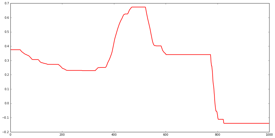

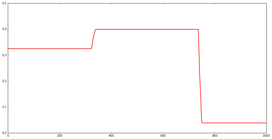
There are interesting subtleties with this model. The path that maximizes the density has mostly zero derivative — while given the exponential distribution of derivatives we would expect zero probability of seeing this. The disconnect comes from maximizing the density rather than sampling from it. If we looked at the paths near the MAP solution I would expect to find mostly non-zero derivatives — the MAP estimate is an extreme point that is not representative of typical samples. This is a general hazard of MAP estimation under heavy-tailed priors.
The Lasso gives the MAP path — the sparse analog of Part I, not of the Kalman filter. The natural question is whether there is a Kalman-like sequential posterior \(P(\mu_t | x_1, \ldots, x_t)\) for the sparse model.
There isn’t, and the reason is concrete: the Gaussian case works because Gaussian likelihood × Gaussian prior = Gaussian posterior, which is fully characterized by two numbers \((a_t, P_t)\) at each step. For the Laplace prior, Gaussian likelihood × Laplace prior produces a posterior that is a complex combination of Gaussian and Laplace terms. Each sequential update compounds this mixture — the resulting distribution has no finite parametrization and cannot be tracked exactly with a recursive filter.
Approximate sequential methods exist (particle filters, expectation propagation), but they sacrifice either exactness or the clean O(T) recursion. The Gaussian model’s tractability is not a minor convenience — it is the direct consequence of conjugacy.